Collaborative Filtering

The algorithm

Collaborative Filtering is a popular technique used in recommendation systems to suggest items or content to users based on their past interactions and the preferences of similar users. It is widely used in various applications, including movie recommendations, product suggestions, music playlists, and more.

The Collaborative Filtering algorithm in the provided module is designed to support various data sources (e.g., S3, Redis, Druid) and different rating mechanisms. It allows users to customize the algorithm by providing options such as the number of days to consider for training, rating values for user-item interactions, thresholds for filtering cold start users and items, and the choice of collaborative filtering algorithm (ALS, Bayesian, or Logistic Matrix Factorization).

How Collaborative Filtering Works

Collaborative Filtering is based on the assumption that users who had similar interests and consumption behaviours in the past will continue having similar tastes in the future. The algorithm uses historical user-item interaction data to find similarities between users or items and make predictions about user preferences for unseen items.

Benefits

• Personalization: Collaborative Filtering provides personalized recommendations to users based on their unique preferences and interactions
• No Need for item metadata: Unlike content-based recommendation systems that require detailed item metadata, Collaborative Filtering solely relies on user-item interaction data, making it more scalable and less dependent on item features
• Serendipity: Collaborative Filtering can introduce users to new items they might not have discovered otherwise, leading to serendipitous recommendations
• Diversity in Recommendations: Implicit collaborative filtering can capture diverse user interests by considering various user interactions with different content. It can recommend less popular or niche content that might be overlooked in explicit rating-based approaches
• No Domain Knowledge Required: Collaborative Filtering does not require domain-specific knowledge about items or users, making it a general-purpose recommendation technique
• Scalability: Public service media platforms typically serve a large number of users and offer a vast catalog of content. Implicit collaborative filtering algorithms can efficiently handle large datasets and scale well with increasing user and item counts

Limitations

• The "cold start" problem: It struggles to make accurate recommendations for new users or items with limited historical data (however with ways to improve situation)
• It can suffer from sparsity issues in the user-item interaction matrix, leading to difficulty in finding similar users or items. Public service media platforms may have sparse and noisy implicit data. Users may not interact with all the content they are interested in, and irrelevant interactions can pollute the data, affecting the quality of recommendations
• Lack of Transparency: The lack of explicit user feedback can make it challenging to understand the reasons behind recommendations. Users might not know why certain content is suggested to them, leading to a lack of transparency in the recommendation process
• Limited Personalization: Implicit collaborative filtering might not provide highly personalized recommendations, especially in scenarios where user behavior is ambiguous or diverse, and no additional demographic or explicit preference data is available
• Popularity Bias: Implicit collaborative filtering tends to recommend popular items more frequently, which can lead to a "rich-get-richer" effect. Lesser-known or niche content may struggle to gain visibility in the recommendation system

Hands on

Preparing dataset

Currently there are multiple supported datasources for preparing dataset, however they would all have similar interface:

from pipe_algorithms_lib.algorithms.cf.data import TrainingData

dataset = TrainingData(
    codops=CODOPS,  # identifier of the organisation
    env='prod',  # environment of source to use data from, either 'dev' or 'prod'
    days=DAYS,  # how many last days we want to use for training
    source='s3',  # see supported options below
    rating=RATING,  # see supported options below
    users_cold_start_threshold=USERS_COLD_START_THRESHOLD,  # any "seldom users" (less than USERS_COLD_START_THRESHOLD unique watched items) would be ignored
    items_cold_start_threshold=ITEMS_COLD_START_THRESHOLD,  # any "unpopular items" (less than ITEMS_COLD_START_THRESHOLD users consumed it in our dataset)
    blacklist_users=BLACKLIST_USERS,  # if we want to blacklist some specific users (e.g. bots), can be list, set, or tuple
    blacklist_items=BLACKLIST_ITEMS,  # if we want to ignore certain items from a dataset, can be list, set, or tuple
    event_type='media_play',  # we want consider any `media_play` event as a user-item interaction

)
dataset.prepare_dataset()

Depending on the parameter env, you either connect to the development or the production environment of the data source, see DEV/PROD environments.

Supported datasources

s3

Reads raw data from "cold storage" in S3 (using pyspark for lazy evaluation). Additional parameters to pass:

• event_type (which event type to consider as interaction, by default it's *, meaning any event type would be considered as interaction, most common value can be media_play or article_start)

redis

Reads processed data from realtime-history. Data pipeline has to be created separately (contact us for the details!). Additional parameters to pass:

• media_type (which media type to consider, in case there are multiple media types supported, e.g. audio, article, or video)

druid

Some sitekeys ingest data into Apache Druid, so it's possible to efficiently retrieve only necessary data using SQL-like queries. Data pipeline has to be created separately (contact us for the details!). Additional parameters to pass:

• datasource (name of the Druid datasource)
• user_id_field (name of the field storing user ID, default client_id)
• media_id_field (name of the field storing media ID, default media_id)
• query (optional, if you want to fully override the default query, must return the result in the same format)

Would generate the following Druid query:

SELECT {user_id_field} AS user_id,
       {media_id_field} AS media_id,
       SUM("count") AS cnt,
       MAX(__time) AS last_play
FROM {datasource}
WHERE TIMESTAMPDIFF(DAY, __time, CURRENT_TIMESTAMP) <= {days}
GROUP BY {user_id_field}, {media_id_field}

Under the hood, they all first load data and convert to a common format, example:

{
    'user1': {'item1': (2, 1690293524), 'item4': (1, 1690293547)},
    'user2': {'item5': (1, 1690293579), 'item1': (1, 1690293591)}
}

where we store information about what items each user has interacted with, keeping also how many times they interacted with it and the timestamp of the last interaction.

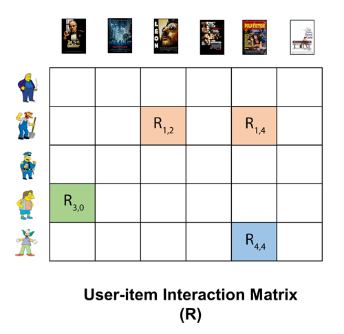
The data preparation step generates a sparse matrix of interactions, with dimensions (num_users, num_items), where most values are 0 (hence sparse) for unobserved items (we don't know if user would like the item or not, we don't have this information) and the other values are computed based on rating function.

We can see schematic representation of such interaction matrix, where each user has one row, and each item has one column.

Supported ratings

Static value

The same fixed value for every user-item interaction. You can pass a value like 42 or 73.1 and it would be used for all non-zero matrix elements

Custom function

If you want to use more elaborated way of computing rating for each user-item interaction, you can provide a function, which as input takes user histories dictionary and returns a dictionary of ratings per each (user_id, item_id), in the following way:

{
    'user1': {'item1': (2, 1690293524), 'item4': (1, 1690293547)},
    'user2': {'item5': (1, 1690293579), 'item1': (3, 1690293591)}
}

->

{
    ('user1', 'item1'): R1,
    ('user1', 'item4'): R2,
    ('user2', 'item5'): R3,
    ('user2', 'item1'): R4,
}

An example of a simple rating function that scales the weight proportionally to number of times the user watched this item:

def my_rating_func(histories):
    ratings = {}
    alpha = 25
    for (user_id, history) in histories.items():
        for (media_id, (cnt, timestamp)) in history.items():
            ratings[(user_id, media_id)] = alpha * cnt
    return ratings

then you just pass reference to the function to TrainingData as TrainingData(..., rating=my_rating_func, ...)

Note

Research on the rating value can be found in the paper Collaborative Filtering for Implicit Feedback Datasets

Training the model

from pipe_algorithms_lib.algorithms.cf.collaborative_filtering import CollaborativeFiltering

model = CollaborativeFiltering(
    codops=CODOPS,  # code of operations. usually implied from a sitekey
    name=MODEL_NAME,  # internal name of the model, e.g. 'personal_episodes'
    algorithm='als',  # supports `als`, `bayesian`, `logistic`
    factors=FACTORS,  # number of hidden features for the model
    iterations=ITERATIONS,  # number of iterations for the algorithm
    env='dev',  # environment in Redis and Milvus, where to save the model, - either 'dev' or 'prod'
    fold_in_rating=40,  # rating to use when estimating embeddings for unknown users (see below); must match the training rating scale
)

model.fit(dataset)  # dataset is the TrainingData object that we prepared before.

Behind the scenes, it's using implicit module. Each algorithm supports some more parameters, like regularization or alpha (can look details in the documentation), which can be passed in the call to CollaborativeFiltering.

The revelant papers describing the algorithms:

• Alternating Least Squares
• Bayesian Personalized Ranking
• Logistic Matrix Factorization

Each of these algorithms has its strengths and weaknesses, and the choice of the most appropriate one depends on factors like the size of the dataset, the sparsity of the data, and the specific requirements of the public service media platform. ALS is a solid choice for scalability and efficiency, while BPR is well-suited for ranking-oriented scenarios. Logistic MF is a good option when direct modeling of user preferences is desired, and the additional computational cost is not prohibitive.

Training step usually takes between 10 minutes and 1 hour, depending on the dataset, algorithm, and hyperparameters.

Info

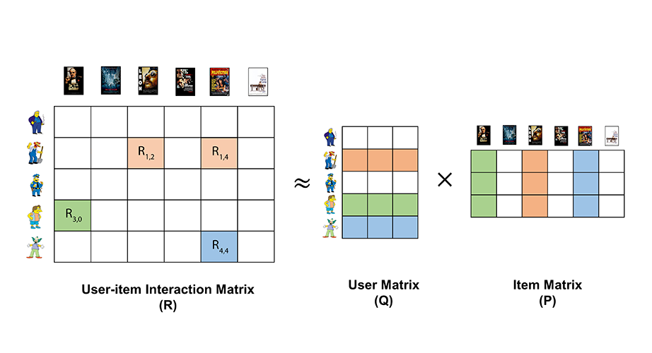
When training the model, we are trying to approximate our interaction matrix with two other matrices, it's called matrix factorization. Matrix factorization helps us to fill in the missing ratings by breaking down this big matrix into two smaller matrices. One matrix represents users and their "hidden" preferences, and the other matrix represents items and their "hidden" characteristics. By multiplying these two smaller matrices together, we can estimate the missing ratings for each user-item combination. The "hidden" preferences and characteristics allow us to capture patterns and similarities among users and items, even if they haven't directly rated or interacted with each other. The vector representing each user is called user embedding and has length factors. The vector representing each item is called item embedding as has the same length factors.

In summary, matrix factorization helps us to predict how much a user might like an item they haven't seen before, based on the relationships between users and items in the past.

Saving the model

After the model has been trained, for each user we have an embedding (fixed-sized vector of numbers with dimensionality FACTORS, representing this user), and each item is also represented by an embedding.

In order to optimize for serving the model to the end user in endpoints, we store these embeddings in the following way:

• user embeddings are stored in Redis hash, since usually we need an embedding for a single user at a time
• item embeddings are stored in Milvus, which is a vector database, optimized for similarity search between vectors

Since storing model is a complex process which potentially can go wrong - we are trying to minimize potential impact on the production endpoint. So that's why when storing model - we create a separate copy, without touching production data. Once the process has been successfully completed, we make a switch and use a new model from now on. This process is called blue-green deployment.

However, you do not need to worry about the details of persisting the model, as the only thing you need to do is to run the following code:

model.save_model()

Serving recommendations

This step is usually done inside the endpoint, any time a user requests a list of recommendations.

Generation of the recommended list happens in the following steps:

1) Extract embedding for a user

2) Compute distance between user embedding and embeddings for all the items. We receive a relevance score, meaning how likely this user would like each item

3) Take first N with the smallest distance (aka the highest relevance), as we are usually interested in top N most relevant items

4) Return recommended items

Steps 2) and 3) are efficiently handled by our vector database engine (Milvus), using Approximate Nearest Neighbors indexing techniques.

In order to generate recommendations for a user, you just run the following code:

model = CollaborativeFiltering(
    codops=CODOPS,
    name=MODEL_NAME,
)

recs = model.recommend(user_id=USER_ID, N=10)

It would return a list of pairs (item_id, score), example: [('item812', 0.721, ('item111', 0.685), ...]

You can do follow-up processing (such as business rules) from now on as you please!

Recommending for users not in the model (fold-in)

It is now possible to get recommendations for users whose embedding was not computed at training time — for example anonymous users, newly registered users, or users from a different context. Instead of (or in addition to) user_id, pass a list of item IDs representing the user's history:

recs = model.recommend(
    user_history_items=['item-a', 'item-b', 'item-c'],
    N=10,
)

If you provide both user_id and user_history_items, the model first tries to look up the stored embedding. If the user is not found (e.g. on a fresh deployment), it falls back to fold-in automatically — so it is always safe to pass both:

recs = model.recommend(
    user_id=USER_ID,
    user_history_items=USER_HISTORY_ITEMS,
    N=10,
)

How it works. At save_model() time, the model stores a compact representation of the full item space (the gram matrix Y^T Y, also called YtY) in Redis alongside the user embeddings. At inference, fold-in uses this matrix together with the vectors of the user's history items to solve the same least-squares problem that ALS would have solved during training — but only for this one user, without touching the trained model. The result is a user embedding placed in the same latent space as all trained users.

Benefits:

• Works for users the model has never seen (anonymous, new, cross-context).
• No retraining or model update needed.
• The embedding is computed from the current history on every request — no stale user state.

Matching the rating scale. The fold-in solve uses the same confidence formula as ALS training (alpha × rating). The fold_in_rating parameter sets the default rating assigned to each item in the history. It must match the scale used at training time:

Training setup	fold_in_rating to set
TrainingData(rating=40) with default alpha=1.0	fold_in_rating=40
TrainingData(rating=1) with alpha=40 on the model	fold_in_rating=1.0 (default)

Using a custom rating function. If you trained with a custom rating function (e.g. recency-weighted), pass the same per-item values at inference time via user_history_ratings. This is a dict of {item_id: rating}. Items absent from the dict fall back to fold_in_rating:

ratings = {
    'item-a': 40,   # high weight
    'item-b': 20,   # lower weight, e.g. older interaction
}

recs = model.recommend(
    user_history_items=list(ratings.keys()),
    user_history_ratings=ratings,
    N=10,
)

Risks and limitations:

• Results are not identical to trained users. Fold-in is an approximation: unlike trained embeddings, which result from joint optimisation across all users and items, fold-in holds all item vectors fixed and optimises only over the new user's history. In practice the difference is small for users with several interactions, but can be more noticeable with very short histories.
• Items not known to the model (not seen during training) are silently skipped. If the entire history consists of unknown items, recommend() returns an empty list.
• Very short histories (1–2 items) produce weaker embeddings — results will resemble item-based similarity more than true personalisation.
• If fold_in_rating or user_history_ratings values don't match the training scale, the embedding will be biased and result quality will degrade.

Related content

Since during training we are creating content embeddings - we can use them to recommend similar items to some specific items! This works by extracting embedding for an input item, compute vector similarity to vectors with all existing items using Milvus and get N items with the highest similarity score. Can use the following code:

model = CollaborativeFiltering(
    codops=CODOPS,
    name=MODEL_NAME,
)

recs = model.recommend_similar_items(item_id, N=10)

Note

Similar items might not be intuitive in this case, since we use Collaborative Filtering to create item embeddings, rather than content based models. So similarity is based purely on content consumption patterns.

Personalizing any list

The collaborative filtering module can be applied in various scenarios to create personalized lists of content for users. Some common use-cases include:

• Personalized Editorial Content: Every platform usually has many editorial content lists and levaraging collaborative filtering is a great way to personalize each list for each user, to match their interests and consuming behaviour. This ensures users receive content that resonates with their preferences at more prominent order, increasing engagement and time spend on the platform.
• Personalized Playlists: Audio and video platforms can employ collaborative filtering to create personalized playlists for users. By analyzing users' listening history and behavior, it can recommend audios or videos that align with their taste, leading to a better user experience and increased user retention.
• Personalized News Feeds: News aggregation platforms can utilize collaborative filtering to deliver personalized news articles to users, even if they are already pre-selected by the editorors. By considering users' reading patterns and interests, the platform can prioritize news stories that are relevant to each user, leading to higher user engagement and satisfaction.

Usage of this functionality within PEACH platform is simple, after doing model training and storing the model, just run:

model.personalize_list(
    user_id='d135176b-1f7b-0a53-57e5-e4971b9205d0',
    ids=['item1', 'item2', 'unknown_item', 'item3', 'item4']
)

As with recommend(), you can pass user_history_items instead of (or as a fallback for) user_id to personalize for users not in the model:

model.personalize_list(
    user_history_items=['item-a', 'item-b', 'item-c'],
    ids=['item1', 'item2', 'unknown_item', 'item3', 'item4']
)

See Recommending for users not in the model above for details on how fold-in works, rating matching, and limitations.

Response format is the same as from model.recommend(). It returns a list of (item_id, score) pairs, where item_id can only be from the input list ids. If the list contains some items unknown to the model - it moves them to the end. Example response:

[
    ('item3', 0.8170211455707),
    ('item2', 0.748350361616138),
    ('item4', 0.671921124564087),
    ('item1', 0.65555475598218206),
    ('unknown_item', -1)
]

Summary

In conclusion, Collaborative Filtering is a powerful and widely used algorithm for generating personalized recommendations based on user-item interaction data. The provided module offers a flexible and modular implementation of item-based Collaborative Filtering, allowing users to customize various parameters and integrate with different data sources to build efficient and accurate recommendation systems.